
Time and Space Complexity
Understanding how algorithms scale with input size.
1. The Intuition
Imagine two algorithms that solve the same problem. Both produce the correct answer, but one takes a fraction of a second while the other takes several minutes when the input becomes large.
Which algorithm is better?
To answer this, we need to understand how an algorithm's resource requirements grow as the input grows.
Consider finding a number in an array:
- Approach A — Linear Search: Check elements one by one.
- Approach B — Binary Search: Repeatedly eliminate half of a sorted array.
For an array of 8 elements, both approaches can be fast. For an array containing one million elements, their performance can differ significantly.
The important question is not simply how fast an algorithm runs today, but how its resource requirements change as the input size increases.
This is the purpose of complexity analysis.
The two resources
| Complexity | What it measures |
|---|---|
| Time complexity | How the number of computational steps grows with input size |
| Space complexity | How the memory requirement grows with input size |
These measures help us compare algorithms independently of a particular machine, programming language implementation, or execution environment.
2. What Is Input Size?
Input size is the quantity of data an algorithm processes. We commonly represent it using (n).
For example:
- An array contains (n) elements.
- A string contains (n) characters.
- A matrix has (n) rows and (m) columns.
- A graph contains (V) vertices and (E) edges.
- An integer may have (n) bits in its binary representation.
The choice of input-size variable depends on the problem.
For an array:
vector<int> nums = {4, 7, 2, 9, 1};
int n = nums.size();
Here, (n=5).
If an algorithm visits every element once, its work grows proportionally to (n).
If it compares every element with every other element, its work may grow proportionally to (n^2).
Always identify what (n) represents before analyzing an algorithm.
3. Time Complexity
Time complexity describes how the number of computational operations grows as a function of input size.
It does not directly measure execution time in seconds. Instead, it studies the growth of the work performed by an algorithm.
Example 1: Constant work
int getFirst(const vector<int>& nums) {
    return nums[0];
}
Assuming the vector is nonempty, the function accesses one element regardless of whether the vector contains 10 or 10 million elements.
Its time complexity is:
[ T(n)=O(1) ]
This is called constant time.
Example 2: One traversal
int sumArray(const vector<int>& nums) {
    int sum = 0;

    for (int x : nums) {
        sum += x;
    }

    return sum;
}
The loop processes all (n) elements once.
If processing each element takes constant time, the total work is proportional to (n).
[ T(n)=O(n) ]
This is called linear time.
Example 3: Nested loops
void printPairs(int n) {
    for (int i = 0; i < n; i++) {
        for (int j = 0; j < n; j++) {
            cout << i << " " << j << '\n';
        }
    }
}
The outer loop runs (n) times. For each outer iteration, the inner loop also runs (n) times.
Therefore, the total number of iterations is:
[ n \times n=n^2 ]
The time complexity is (O(n^2)).
Key idea: Count how the work grows, not merely how many loops appear in the code.
4. Asymptotic Notation
Asymptotic notation describes the growth of a function as input size becomes large. It lets us ignore implementation-specific details and focus on the dominant growth pattern.
Three important notations are Big O, Big Omega, and Big Theta.
Big O — (O)
Big O describes an asymptotic upper bound on growth.
Informally, (T(n)=O(n^2)) means that, beyond some input size, the function is bounded above by a constant multiple of (n^2).
In algorithm discussions, Big O is frequently used to express worst-case complexity, but these concepts are not identical. Big O itself does not automatically mean worst case.
Big Omega — (\Omega)
Big Omega describes an asymptotic lower bound on growth.
For example, (T(n)=\Omega(n)) means that the function grows at least as fast as a constant multiple of (n), for sufficiently large (n).
Big Theta — (\Theta)
Big Theta describes a tight asymptotic bound: both an upper and a lower bound of the same growth order.
If an algorithm performs work proportional to (n), then its time complexity is (\Theta(n)).
A practical example
Suppose the exact number of operations is:
[ T(n)=3n^2+5n+10 ]
For large (n), the quadratic term dominates the linear and constant terms.
Thus:
[ T(n)=\Theta(n^2) ]
It is also correct to say (T(n)=O(n^2)) and (T(n)=\Omega(n^2)).
Rules for simplifying complexity
When finding the dominant asymptotic growth:
- Ignore constant multiplicative factors.
- Ignore lower-order terms when a higher-order term dominates.
- Keep different input variables when they represent independent dimensions.
Examples:
| Expression | Tight bound |
|---|---|
| (7n+20) | (\Theta(n)) |
| (4n^2+3n+8) | (\Theta(n^2)) |
| (6n^3+100n^2) | (\Theta(n^3)) |
| (12\log_2 n+5) | (\Theta(\log n)) |
| (n\log n+4n) | (\Theta(n\log n)) |
Remember: removing lower-order terms is appropriate for asymptotic analysis, not for calculating an exact operation count.
5. Common Time Complexities
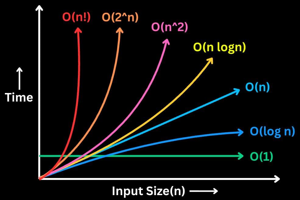
The following table shows common growth rates, ordered approximately from slower growth to faster growth.
| Complexity | Name | Typical example |
|---|---|---|
| (O(1)) | Constant | Array indexing |
| (O(\log n)) | Logarithmic | Binary search |
| (O(\sqrt n)) | Square-root | Trial division up to (\sqrt n) |
| (O(n)) | Linear | Linear search |
| (O(n\log n)) | Linearithmic | Merge sort |
| (O(n^2)) | Quadratic | All pairs in an array |
| (O(n^3)) | Cubic | Three nested linear loops |
| (O(2^n)) | Exponential | Generating all subsets |
| (O(n!)) | Factorial | Generating all permutations |
These are typical patterns, not universal classifications of every algorithm that uses the corresponding technique.
How growth changes
Consider an input size of (n=1{,}000).
- (O(1)): a constant amount of work.
- (O(\log_2 n)): approximately 10 logarithmic steps.
- (O(n)): roughly 1,000 units of work.
- (O(n^2)): roughly 1,000,000 units of work.
- (O(2^n)): an astronomically large number of possibilities.
The values above are illustrative growth comparisons, not guaranteed execution times or exact operation counts.
The practical lesson is that an algorithm that works well on small inputs may become unusable as the input grows.
6. Analyzing Loops
Loop analysis is one of the most useful skills in DSA.
Pattern A: A single linear loop
for (int i = 0; i < n; i++) {
    // Constant-time work
}
Iterations: (n).
[ T(n)=\Theta(n) ]
Pattern B: Two consecutive loops
for (int i = 0; i < n; i++) {
    // Constant-time work
}

for (int j = 0; j < n; j++) {
    // Constant-time work
}
Total iterations:
[ n+n=2n ]
Therefore:
[ T(n)=\Theta(n) ]
Consecutive loops add their work; they do not automatically multiply their complexities.
Pattern C: Two nested loops
for (int i = 0; i < n; i++) {
    for (int j = 0; j < n; j++) {
        // Constant-time work
    }
}
Total iterations:
[ n \cdot n=n^2 ]
Therefore:
[ T(n)=\Theta(n^2) ]
Pattern D: A triangular loop
for (int i = 0; i < n; i++) {
    for (int j = 0; j <= i; j++) {
        // Constant-time work
    }
}
The inner loop does not run (n) times on every iteration. It runs (1,2,3,\ldots,n) times.
Total iterations:
[ 1+2+\cdots+n=\frac{n(n+1)}{2} ]
After simplifying:
[ T(n)=\Theta(n^2) ]
The upper bound is quadratic even though the number of iterations differs from a full (n \times n) nested loop.
Pattern E: A loop that doubles
for (int i = 1; i < n; i *= 2) {
    // Constant-time work
}
The values of i are approximately:
[ 1,2,4,8,16,\ldots ]
After (k) iterations, i is approximately (2^k). The loop stops when it reaches (n).
[ 2^k \ge n ]
Taking logarithms gives:
[ k \ge \log_2 n ]
Therefore:
[ T(n)=\Theta(\log n) ]
Pattern F: A loop that halves
for (int i = n; i > 0; i /= 2) {
    // Constant-time work
}
The values decrease approximately as:
[ n,\frac n2,\frac n4,\frac n8,\ldots ]
The loop performs logarithmically many iterations:
[ T(n)=\Theta(\log n) ]
Pattern G: Nested logarithmic loops
for (int i = 1; i < n; i *= 2) {
    for (int j = 1; j < n; j *= 2) {
        // Constant-time work
    }
}
Each loop runs (\Theta(\log n)) times.
[ T(n)=\Theta(\log n\cdot\log n) ]
Therefore:
[ T(n)=\Theta((\log n)^2) ]
Pattern H: A loop with a dependent bound
for (int i = 1; i < n; i *= 2) {
    for (int j = 0; j < i; j++) {
        // Constant-time work
    }
}
The inner loop runs (1,2,4,8,\ldots) times.
Its total work is:
[ 1+2+4+\cdots+2^k ]
For a geometric series, the sum is dominated by its largest term. Since that term is proportional to (n), the total work is (\Theta(n)), not (\Theta(n\log n)).
This is an important pattern: the number of outer iterations alone does not determine the total work.
7. Best, Average, and Worst Cases
An algorithm may perform different amounts of work on different inputs of the same size.
Consider linear search.
int linearSearch(const vector<int>& nums, int target) {
    for (int i = 0; i < nums.size(); i++) {
        if (nums[i] == target) {
            return i;
        }
    }

    return -1;
}
Best case
The target is the first element. Only one comparison is required.
[ T_{\text{best}}(n)=\Theta(1) ]
Worst case
The target is the last element, or it does not exist. The algorithm may inspect every element.
[ T_{\text{worst}}(n)=\Theta(n) ]
Average case
The average depends on the distribution of inputs and the assumptions used.
If the target is guaranteed to occur and is equally likely to occupy any position, the expected number of comparisons is:
[ \frac{1+2+\cdots+n}{n}=\frac{n+1}{2} ]
Therefore, under this assumption:
[ T_{\text{average}}(n)=\Theta(n) ]
If the target can be absent, the average changes depending on the probability that it is absent and how present targets are distributed.
Best, average, and worst cases describe different input scenarios. Big O, Omega, and Theta describe bounds on a function. They should not be treated as interchangeable terms.
8. Space Complexity
Space complexity describes how memory usage grows with input size.
It is useful to distinguish two measurements:
- Total space: All memory used by the algorithm, including storage for its input.
- Auxiliary space: Additional memory used by the algorithm beyond the input storage, under the convention being used.
In many DSA discussions, auxiliary space is the more useful comparison because the input may already exist before the algorithm starts.
Example 1: Constant auxiliary space
int findMax(const vector<int>& nums) {
    int maximum = nums[0];

    for (int x : nums) {
        maximum = max(maximum, x);
    }

    return maximum;
}
The algorithm uses a fixed number of extra variables.
[ S_{\text{aux}}(n)=\Theta(1) ]
The input contains (n) elements, so its storage is (\Theta(n)). If we include the input in the total, the overall storage is (\Theta(n)).
Example 2: An extra array
vector<int> copyArray(const vector<int>& nums) {
    vector<int> copy = nums;
    return copy;
}
The copied array stores (n) elements.
[ S_{\text{aux}}(n)=\Theta(n) ]
If the input is also counted, total storage is still (\Theta(n)), although the actual memory requirement is larger than that of the first example.
Example 3: A two-dimensional matrix
vector<vector<int>> matrix(n, vector<int>(n, 0));The matrix stores (n^2) elements.
[ S(n)=\Theta(n^2) ]
The same reasoning applies to a square DP table or an adjacency matrix.
Example 4: In-place modification
void reverseArray(vector<int>& nums) {
    int left = 0;
    int right = static_cast<int>(nums.size()) - 1;

    while (left < right) {
        swap(nums[left], nums[right]);
        left++;
        right--;
    }
}
The array is modified directly, using only a few additional variables.
[ S_{\text{aux}}(n)=\Theta(1) ]
In-place does not necessarily mean that absolutely no extra memory is used. It usually means that the algorithm operates within the existing data structure using a small amount of auxiliary storage.
9. Recursion and the Call Stack
Recursive functions consume stack space because each active function call needs its own execution state.
Example 1: Linear recursion
int factorial(int n) {
    if (n <= 1) return 1;
    return n * factorial(n - 1);
}
The function makes (n) calls before reaching the base case.
Each call performs constant work apart from the recursive call.
Time complexity:
[ T(n)=\Theta(n) ]
Maximum recursion depth:
[ S_{\text{stack}}(n)=\Theta(n) ]
Example 2: Tail recursion
int factorialTail(int n, int result = 1) {
    if (n <= 1) return result;
    return factorialTail(n - 1, result * n);
}
The logical work remains linear, and the recursion depth is linear.
Time complexity:
[ T(n)=\Theta(n) ]
Stack space in a typical C++ execution without guaranteed tail-call elimination:
[ S_{\text{stack}}(n)=\Theta(n) ]
Do not automatically assume that tail recursion uses constant stack space in C++. C++ does not guarantee tail-call optimization.
Example 3: Binary search
int binarySearch(const vector<int>& nums, int target,
                 int left, int right) {
    if (left > right) return -1;

    int mid = left + (right - left) / 2;

    if (nums[mid] == target) return mid;

    if (nums[mid] < target) {
        return binarySearch(nums, target, mid + 1, right);
    }

    return binarySearch(nums, target, left, mid - 1);
}
Each call eliminates approximately half the remaining search range.
Time complexity:
[ T(n)=\Theta(\log n) ]
Auxiliary stack space:
[ S_{\text{stack}}(n)=\Theta(\log n) ]
An iterative binary search can retain the same time complexity while using (\Theta(1)) auxiliary space.
10. Recurrence Relations
A recurrence describes the work of a recursive algorithm in terms of smaller inputs.
A common example is:
[ T(n)=T(n-1)+\Theta(1) ]
Each call solves a problem one unit smaller and performs constant additional work.
Expanding the recurrence gives:
[ T(n)=T(n-2)+\Theta(1)+\Theta(1) ]
Continuing until the base case yields:
[ T(n)=\Theta(n) ]
Binary search recurrence
[ T(n)=T(n/2)+\Theta(1) ]
Each step halves the problem size and does constant additional work.
The number of halvings is logarithmic, so:
[ T(n)=\Theta(\log n) ]
Merge sort recurrence
Merge sort divides the array into two halves, recursively sorts each half, and merges the results in linear time.
[ T(n)=2T(n/2)+\Theta(n) ]
There are approximately (\log_2 n) levels of recursion. At each level, the combined merging work is (\Theta(n)).
Therefore:
[ T(n)=\Theta(n\log n) ]
Its auxiliary space is typically (\Theta(n)) for the merge buffer, excluding implementation-specific details.
A useful recurrence pattern
For divide-and-conquer algorithms, the Master Theorem can often help solve recurrences of the form:
[ T(n)=aT(n/b)+f(n) ]
where (a) is the number of recursive subproblems, (n/b) is their approximate size, and (f(n)) is the work outside the recursive calls.
It is a powerful tool, but it applies under specific conditions; not every recurrence can be solved directly with it.
11. Complexity of Familiar DSA Algorithms
| Algorithm | Time complexity | Auxiliary space |
|---|---|---|
| Array traversal | (\Theta(n)) | (\Theta(1)) |
| Linear search | (O(n)) worst case | (\Theta(1)) |
| Iterative binary search | (O(\log n)) worst case | (\Theta(1)) |
| Bubble sort, optimized | (O(n)) best, (O(n^2)) worst | (\Theta(1)) |
| Merge sort on arrays | (\Theta(n\log n)) | (\Theta(n)) |
| Heap sort | (\Theta(n\log n)) | (O(1)) auxiliary for standard in-place implementation |
| Kadane's algorithm | (\Theta(n)) | (\Theta(1)) |
| Moore's Voting Algorithm | (\Theta(n)) | (\Theta(1)) |
These are standard bounds under conventional implementations and assumptions. For example, the optimized bubble sort best case is linear when it stops after a pass with no swaps.
Connecting complexity to Kadane's algorithm
Kadane's algorithm finds the maximum sum of a contiguous subarray by maintaining a running sum and the best answer so far.
For each element, it performs a constant amount of work.
int maxSubArray(const vector<int>& nums) {
    int current = nums[0];
    int best = nums[0];

    for (int i = 1; i < nums.size(); i++) {
        current = max(nums[i], current + nums[i]);
        best = max(best, current);
    }

    return best;
}
It traverses the array once:
[ T(n)=\Theta(n) ]
It stores only two running values and uses no input-sized auxiliary structure:
[ S_{\text{aux}}(n)=\Theta(1) ]
This is an example of an efficient algorithm that achieves linear time with constant auxiliary space.
12. Common Problem-Solving Patterns
Pattern 1: One pass
If every element is processed a constant number of times, the time complexity is generally (\Theta(n)).
Examples: computing a sum, finding a maximum, and Kadane's algorithm.
Pattern 2: Pairwise comparisons
Comparing every element against every other element usually requires quadratic work.
Examples: brute-force duplicate detection and checking all pairs.
For an array of (n) elements, the number of unique pairs is:
[ \frac{n(n-1)}{2}=\Theta(n^2) ]
Pattern 3: Repeated halving
If the remaining problem size is repeatedly divided by a constant factor, the number of stages is generally logarithmic.
Examples: binary search and many balanced divide-and-conquer algorithms.
Pattern 4: Sorting followed by scanning
Sorting an array typically costs (O(n\log n)), while a subsequent linear scan costs (O(n)).
Together:
[ O(n\log n)+O(n)=O(n\log n) ]
This is a common trade-off: extra sorting work may make a problem easier to solve or reduce the need for nested loops.
Pattern 5: Precomputation and lookup
Building a prefix-sum array takes (\Theta(n)) time and (\Theta(n)) extra space. Once built, a range-sum query can be answered in (\Theta(1)) time.
This illustrates an important algorithm-design principle: spend additional time or memory up front to make repeated operations cheaper.
13. Common Mistakes
Mistake 1: Assuming every nested loop is (O(n^2))
A nested loop may have a dependent bound or logarithmic iteration count. Analyze the actual number of iterations rather than counting loops.
Mistake 2: Multiplying consecutive loops
Two separate loops of length (n) perform (2n) iterations, not (n^2).
Mistake 3: Treating Big O as exact runtime
(O(n)) does not mean an algorithm takes exactly (n) seconds or performs exactly (n) instructions. It expresses an upper bound on asymptotic growth.
Mistake 4: Ignoring recursive stack space
An algorithm that creates no arrays may still use linear or logarithmic memory through recursion.
Mistake 5: Confusing total space with auxiliary space
Always state whether input storage is included. This is particularly important when comparing in-place algorithms with algorithms that allocate additional arrays.
Mistake 6: Assuming all (O(n\log n)) algorithms perform identically
Constants, memory access patterns, allocations, cache behavior, and implementation details can influence actual performance.
Mistake 7: Assuming the most complex-looking expression determines the answer
For (3n^2+100n), the quadratic term dominates asymptotically. For (n\log n+50n), the (n\log n) term dominates.
Mistake 8: Using (n) for every dimension
For an (n \times m) matrix, a full traversal takes (\Theta(nm)), not necessarily (\Theta(n^2)).
Mistake 9: Assuming in-place means zero extra memory
A few pointers, counters, and temporary variables still occupy memory. In-place algorithms generally aim to keep auxiliary space small.
Mistake 10: Confusing input size with numeric value
An algorithm that processes the binary digits of an integer (N) may run in (\Theta(\log N)) time, because the number of binary digits grows logarithmically with (N).
14. Practice Problems
Try each problem before revealing its solution. Focus on explaining why the complexity has that growth rate.
Problem 1 — Consecutive loops
What is the time complexity?
for (int i = 0; i < n; i++) {
    cout << i;
}

for (int j = 0; j < n; j++) {
    cout << j;
}▶Reveal answer
Each loop performs (n) iterations. The total is (n+n=2n).
Time: (\Theta(n))
Problem 2 — Triangular loop
Determine the time complexity.
for (int i = 1; i <= n; i++) {
    for (int j = 1; j <= i; j++) {
        cout << j;
    }
}▶Reveal answer
The inner loop runs (1,2,\ldots,n) times across the outer iterations.
[ T(n)=\sum_{i=1}^{n}i=\frac{n(n+1)}{2} ]
Time: (\Theta(n^2))
Problem 3 — Doubling loop
Determine the time complexity.
for (int i = 1; i < n; i *= 2) {
    cout << i;
}▶Reveal answer
The loop variable doubles each iteration. It reaches the stopping threshold after approximately (\log_2 n) iterations.
Time: (\Theta(\log n))
Problem 4 — Dependent inner loop
Determine the time complexity.
for (int i = 1; i < n; i *= 2) {
    for (int j = 0; j < i; j++) {
        cout << j;
    }
}▶Reveal answer
The inner loop executes (1,2,4,8,\ldots) times. The sum of these powers of two is bounded by a constant multiple of (n).
Time: (\Theta(n))
Problem 5 — Auxiliary space
What is the auxiliary space complexity?
int calculate(const vector<int>& nums) {
    int sum = 0;

    for (int x : nums) {
        sum += x;
    }

    return sum;
}▶Reveal answer
The function stores only a fixed number of variables and does not allocate additional memory proportional to the input.
Auxiliary space: (\Theta(1))
The input itself occupies (\Theta(n)) storage, if input storage is included in the total-space measurement.
Problem 6 — Recursive countdown
Analyze both time and auxiliary stack space.
void countdown(int n) {
    if (n <= 0) return;

    countdown(n - 1);
}▶Reveal answer
There are linearly many recursive calls, each doing constant work.
Time: (\Theta(n))
The maximum active recursion depth is proportional to (n).
Auxiliary stack space: (\Theta(n))
Problem 7 — Two input dimensions
A function traverses every cell in a matrix with (n) rows and (m) columns. What is its time complexity?
▶Reveal answer
Each of the (n) rows contains (m) cells, so the total number of cells is (nm).
Time: (\Theta(nm))
It simplifies to (\Theta(n^2)) only under an assumption such as (m=n).
Problem 8 — Binary search versus linear search
For a sorted array of (n) elements, compare the worst-case time complexity of iterative binary search and linear search.
▶Reveal answer
Linear search may inspect every element, giving (O(n)) worst-case time.
Binary search halves the remaining search range on each iteration, giving (O(\log n)) worst-case time.
For sufficiently large inputs, logarithmic growth is much slower than linear growth.
15. Quick Reference Cheat Sheet
| Code or operation pattern | Typical complexity |
|---|---|
| Fixed number of operations | (\Theta(1)) |
| One complete traversal | (\Theta(n)) |
| Two consecutive traversals | (\Theta(n)) |
| Two full nested loops | (\Theta(n^2)) |
| Three full nested loops | (\Theta(n^3)) |
| Repeated doubling or halving | (\Theta(\log n)) |
| Two nested logarithmic loops | (\Theta((\log n)^2)) |
| Divide-and-conquer with two half-size calls and linear combine work | (\Theta(n\log n)), under the usual recurrence assumptions |
| Extra array of (n) elements | (\Theta(n)) auxiliary space |
| Recursion depth proportional to (n) | (\Theta(n)) stack space |
| Fixed number of auxiliary variables | (\Theta(1)) auxiliary space |
A reliable analysis checklist
When analyzing a new algorithm, ask:
- What does the input size represent?
- How many times does each loop execute?
- Are loops consecutive, nested, or dependent on one another?
- Does recursion reduce the input by one, divide it, or create multiple subproblems?
- What is the best-, average-, or worst-case scenario being analyzed?
- What extra memory is allocated?
- How much memory does the recursion stack require?
- Which term dominates as the input becomes large?
- Am I reporting total space or auxiliary space?
- Have I stated the assumptions behind the result?
16. Final Takeaway
Time and space complexity help us reason about the scalability of algorithms before relying on benchmarks or machine-specific execution times.
The most important skill is not memorizing complexity classes. It is learning to derive them from the structure of the code, the input size, the operations performed, and the memory used.
As you practice DSA, make it a habit to analyze both time and auxiliary space after solving each problem. Over time, recognizing these patterns becomes much more natural.